Ant Colony Optimization to solve a classic Asymmetric Travelling Sales Man Problem

A python implementation of an ant colony optimization algorithm with offline pheromone update to solve ry48p, an asymmetric travelling sales man problem

Introduction

Travelling Sales Man (TSP) is a class of optimization problems in computer science which are solved by finding the best solutions out of a very large discrete solution set. TSP can be described easily with the analogy of a sales man travelling to N cities with least possible distance. The term asymmetric implies that the distance between A to B may be different from B to A. The concept of TSP can be applied to various real-world applications like network routing, logistics, etc. (Further information on TSP can be found athttp://simple.wikipedia.org/wiki/Travelling_salesman_problem).

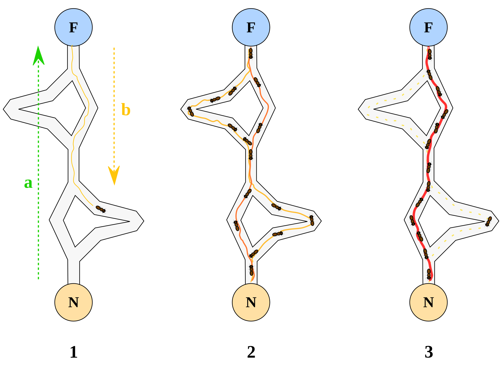
Ant Colony Optimization (ACO) is one of the computational intelligence techniques that can be used to solve a Travelling Sales Man problem. ACO is inspired by the ability (using stigmergy) of ants to find the shortest path between their colony and a food source. In this computational technique, we probabilistically build a solution by systematically adding smaller sub components. The solution thus built is evaluated based on meta-heuristics, and the evaluation result is applied as a feedback to the next iteration. The solution is thus improved over N iterations with the help of feedback from the previous iterations.

In this article, I have explained a python implementation of ACO for solving an asymmetric travelling sales man problem. The input data I have used is a commonly used ry48p dataset. The best solution for ry48p as published in TSP site is 14422 though I managed to reach only 15473. But considering the stochastic nature of algorithms, this algorithm can even give a better solution. I have also published results for experiments that were conducted to test the performance of the algorithm with different parameter values. All the experimental results were derived by averaging out of 20 trial runs.

Background

Ant Colony Optimization was first introduced by Dorigo in 1992, so it is relatively a new technology compared to other computational intelligence techniques. Real life studies were conducted on ants to study their logistic behaviour. Deneubourg has published an article describing such characteristics of the ants in his paper on Double Bridge experiment. The experiment was originally executed using a laboratory colony of Argentine ants. It is known that these ants deposit pheromone both when leaving and returning to the nest. As a result of the experiment, it was discovered that the ants use their pheromone strength as a means of communicating shortest possible distance between their nest and food source to other ants.

Using the Code

Source Code is available for download at https://aco-travelling-salesman.googlecode.com/files/aco-travelling-salesman.zip

The algorithm is initialized with the following parameters:

• Ant_count: Numbers of ants that will be exploring the population
• Iterations: Number of generations for which ants will be searching for solutions
• PheromoneConstant: The constant used as a sufficient while calculating strength of pheromone applied by an individual ant based on its tour length
• DecayConstant: Strength with which pheromone decays in a path
• Alpha: Pheromone strength while finding the next city
• Beta: Heuristic strength while finding the next city
• Initialization: How to initialize first population, either random or with a specific city

 Collapse | Copy Code

# Algorithm paramters
ant_count = 10
iterations = 500
PheromoneConstant = 1.0
DecayConstant = 0.2
Alpha = 1   # Pheromone constant
Beta = 1   # Heuristic constant

RANDOM = 1
CITY0 = 0 
initialization = RANDOM

Function readTsp() is responsible for reading the input data. Currently, it parses a text file containing data in the standard ry48p format. This function can be easily modified to read data in any format as one wish.

 Collapse | Copy Code

def readTsp():
   pathmatrix = []
   tspfile = open('tsp_matrix.atsp', 'r')
   for cities in range(48):
      city = []

      line1 = tspfile.readline()
      for node in line1.split():
         city.append(int(node.strip()))

      line1 = tspfile.readline()
      for node in line1.split():
         city.append(int(node.strip()))

      line1 = tspfile.readline()
      for node in line1.split():
         city.append(int(node.strip()))

      line1 = tspfile.readline()
      for node in line1.split():
         city.append(int(node.strip()))
      
      pathmatrix.append(city)
return pathmatrix

The core functionality of the algorithm is coded in the method "def shortestPath(cities_matrix, ant_count, iterations)". In the inner for-loop, each ant in the colony finds the next available node in the graph based on heuristics and pheromone strength. After all the ants have moved to the next available node, the pheromone is updated over the traversed path. The outer while-loop will now iterate to repeat the same process until all the ants have reached their destination. Once all the ants have reached the destination, the outermost for-loop will iterate for as many number of iterations specified in the algorithm parameters. Result is taken from the best solution of each iteration.

 Collapse | Copy Code

for iteration in range(iterations):

   # Initialize ants with a random city
   paths = initialize_ants(ant_count,cities_count)

   while not isAllCompletedTour(paths,cities_count):   # End iteration when all ants have completed the tour
      # For each ant in the colony
      for ant in range(ant_count):   

         # Termination criteria
         if len(paths[ant]) < cities_count:
               
            paths[ant].append(nextCity(cities_matrix, pheromone_trail,paths[ant]))   # Find next town

   # After all ants have completed the tour - Update pheromone
   updatePheromone(pheromone_trail, paths,cities_matrix)
   (globalBest,path) = iterationResult(iteration,paths,cities_matrix,(globalBest,path))

Points of Interest

Following experiments were conducted to test the performance of the algorithm with different parameter values. All the experimental results were derived by averaging out of 20 trial runs.

Experiment 1: Optimal Ant Count and Iteration

There is no well-defined value in the literature that suggests a right value for ant count and iterations. Therefore I have carried out an experiment to test the best combinations of ant count and iteration. The list of values used for ant_count are 1,10,50,100,150,200. The list of values used for iterations are 10,50,100,250,500,1000. All the 36 combinations from the list are experimented and the interesting values alone from the experiment are plotted in Figure 1.

Figure 1: Experiment1 – convergence of ant_count and iteration

As we can see in Figure 1, the algorithm is performing better with increase in ant count. A single ant is certainly not able to converge to any better solution, but it explores the search space randomly and gives random solutions. As we increase the ant counts, the algorithm is certainly moving to a convergence. For an ant count of 10 it is converging around 70 and for an ant count of 50 it is converging around 20. While further increasing the ant count value to 100 and 200, the convergence is achieved around 10 iterations, in such case it may not be worth considering any big ant count size.

Regarding the number of iterations, as we can see from Fig 1 that the convergence lies in the range of 10 to 25 for sufficiently large ant counts (50 and above). Only increasing the iterations can increase the probability of an ant exploring to a new random solution but convergence will remain the same.

Figure 2a and 2b compares the computational overhead of the two variables ant count and iterations respectively. It is identified from these graphs that the executions times are directly proportional to the variables and increase linearly along with the variables.

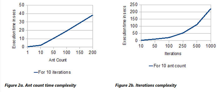Therefore considering the convergence and execution time analysis of ant count and iterations, it appears that anant_count of 50 running for 200 iterations will be enough to solve this problem.

Experiment 2: Analysis of Decay Constant Analysis

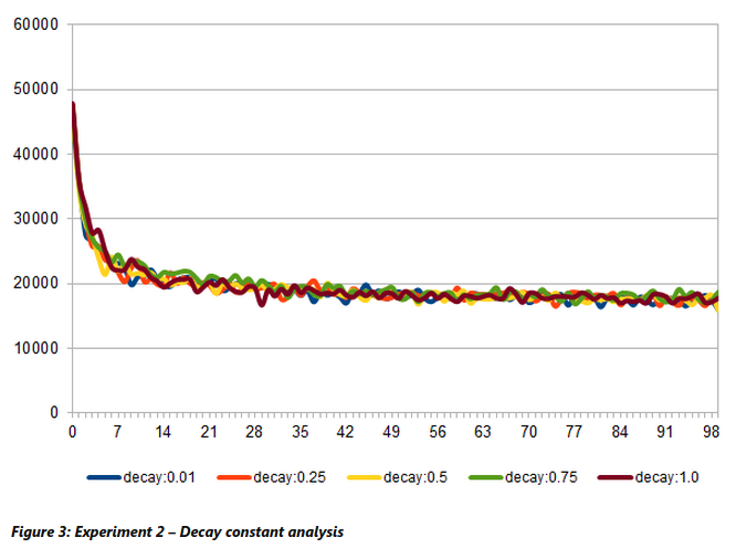
This experiment compares the convergence time of the algorithm against various value for decay constants. Five values were originally considered for analysing decay constants, they are 0.01, 0.25, 0.5, 0.75 and 1.0. The results are shown in Figure 3. Decay value of 1 means that no previous values are preserved and only the n-1^th round pheromone is used.

As we could see, decay constant of 1.0 took a long time to refine the results. On the other hand, a decay constant of 0.01 means there is very little evaporation and hence there is less exploration in the search space. It appears from the trend that an optimal value could be 0.25 because it shows a reasonable exploitation (gradual improvement) as well as occasional exploration (bumps).

Experiment 3: Analysing Pheromone Constant

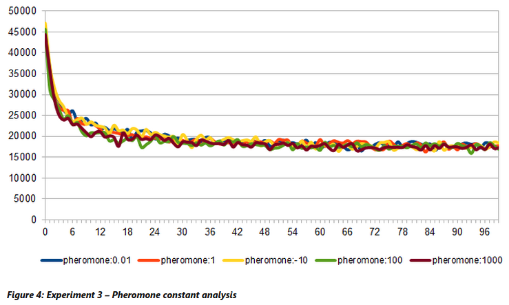
This experiment compares the convergence time of the algorithm against various values for pheromone constants. Five values that were used for analysing pheromone constant are 0.01,1,10,100,1000. It is quite clear from Figure 4 that a higher pheromone constant of 100 and 1000 are causing a quicker convergence. This is mainly because increasing the pheromone constant will indirectly increase the pheromone strength in the path and hence leads to convergence.

Experiment 4: Alpha Beta Analysis

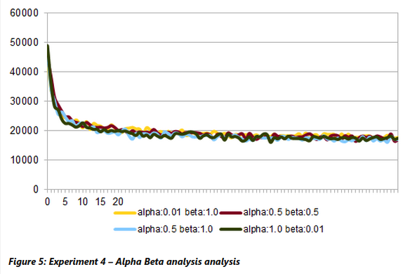
The Alpha controls the strength of pheromone in choosing the path while Beta controls the strength of heuristic in choosing the path. It is seems from Figure 5 that trends with higher alpha value and lower beta value show a better convergence than trends with lower alpha value and higher beta value.

History

• 20^th December, 2014: Initial version

• License

  This article, along with any associated source code and files, is licensed under The Code Project Open License (CPOL)

writer: Pravin baskaran

source